
| 일 | 월 | 화 | 수 | 목 | 금 | 토 |
|---|---|---|---|---|---|---|
| 1 | 2 | 3 | 4 | 5 | ||
| 6 | 7 | 8 | 9 | 10 | 11 | 12 |
| 13 | 14 | 15 | 16 | 17 | 18 | 19 |
| 20 | 21 | 22 | 23 | 24 | 25 | 26 |
| 27 | 28 | 29 | 30 |
Tags
- Kafka
- token filter test
- analyzer test
- 차트
- license delete
- License
- licence delete curl
- docker
- Java
- Elasticsearch
- zip 암호화
- ELASTIC
- flask
- plugin
- API
- springboot
- query
- TensorFlow
- 파이썬
- matplotlib
- Test
- Python
- aggs
- 900gle
- aggregation
- MySQL
- zip 파일 암호화
- Mac
- sort
- high level client
Archives
- Today
- Total
개발잡부
[es] 검색결과 비교 - score 본문
반응형
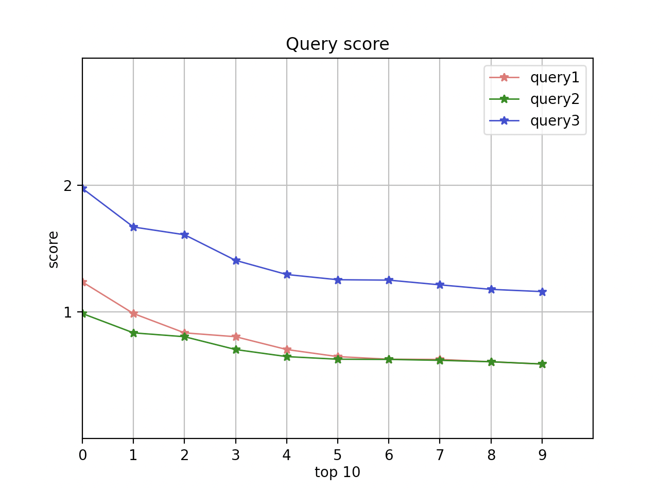
무쓸모 쿼리 결과 스코어 차트를 만들었다. 이 쓸모없는 것을 활용해보잣
https://ldh-6019.tistory.com/201?category=1029507
[es] 검색결과를 검증해보자
True Positive(TP) : 실제 True인 정답을 True라고 예측 (정답) False Positive(FP) : 실제 False인 정답을 True라고 예측 (오답) False Negative(FN) : 실제 True인 정답을 False라고 예측 (오답) True Negative(..
ldh-6019.tistory.com
1. 같은 쿼리에 부스팅을 다르게 줘서 score 변화를 비교한다.
case 1 : category에 ^2 - query 1
case 2 : 부스팅 X - query 2
case 3 : name에 ^2 - query 3
결과
query_mat.py
# -*- coding: utf-8 -*-

import time
import math

from elasticsearch import Elasticsearch

import tensorflow_hub as hub
import tensorflow_text

import matplotlib.pyplot as plt
import numpy as np

##### SEARCHING #####

def get_result(script_query):
    response = client.search(
        index=INDEX_NAME,
        body={
            "size": SEARCH_SIZE,
            "query": script_query,
            "_source": {"includes": ["name", "category"]}
        }
    )

    return [hit["_score"] for hit in response["hits"]["hits"]]

def handle_query():
    query = "나이키 남성 신발"
    query_vector = embed_text([query])[0]

    script_query1 = {
        "function_score": {
            "query": {
                "multi_match": {
                    "query": query,
                    "fields": [
                        "name",
                        "category^2"
                    ]
                }
            },
            "functions": [
                {
                    "script_score": {
                        "script": {
                            "source": "cosineSimilarity(params.query_vector, 'feature_vector') * doc['weight'].value * doc['popular'].value / doc['name.keyword'].length + doc['category.keyword'].length",
                            "params": {
                                "query_vector": query_vector
                            }
                        }
                    },
                    "weight": 0.1
                }
            ]
        }
    }

    script_query2 = {
        "function_score": {
            "query": {
                "multi_match": {
                    "query": query,
                    "fields": [
                        "name",
                        "category"
                    ]
                }
            },
            "functions": [
                {
                    "script_score": {
                        "script": {
                            "source": "cosineSimilarity(params.query_vector, 'feature_vector') * doc['weight'].value * doc['popular'].value / doc['name.keyword'].length + doc['category.keyword'].length",
                            "params": {
                                "query_vector": query_vector
                            }
                        }
                    },
                    "weight": 0.1
                }
            ]
        }
    }


    script_query3 = {
        "function_score": {
            "query": {
                "multi_match": {
                    "query": query,
                    "fields": [
                        "name^2",
                        "category"
                    ]
                }
            },
            "functions": [
                {
                    "script_score": {
                        "script": {
                            "source": "cosineSimilarity(params.query_vector, 'feature_vector') * doc['weight'].value * doc['popular'].value / doc['name.keyword'].length + doc['category.keyword'].length",
                            "params": {
                                "query_vector": query_vector
                            }
                        }
                    },
                    "weight": 0.1
                }
            ]
        }
    }

    # print(response["hits"]["max_score"])
    x = np.arange(0, SEARCH_SIZE, 1)
    y1 = get_result(script_query1)
    y2 = get_result(script_query2)
    y3 = get_result(script_query3)

    plt.xlim([1, SEARCH_SIZE])      # X축의 범위: [xmin, xmax]
    plt.ylim([0, MAX_SCORE])     # Y축의 범위: [ymin, ymax]
    plt.xlabel('top 10', labelpad=2)
    plt.ylabel('score', labelpad=2)
    plt.plot(x, y1, label='query1', color='#e35f62', marker='*', linewidth=1 )
    plt.plot(x, y2, label='query2', color='#008000', marker='*', linewidth=1 )
    plt.plot(x, y3, label='query3', color='#3333cc', marker='*', linewidth=1 )

    plt.legend()
    plt.title('Query score')
    plt.xticks(x)
    plt.yticks(np.arange(1, MAX_SCORE))
    plt.grid(True)
    plt.show()

##### EMBEDDING #####

def embed_text(input):
    vectors = model(input)
    return [vector.numpy().tolist() for vector in vectors]


##### MAIN SCRIPT #####

if __name__ == '__main__':
    INDEX_NAME = "goods"

    SEARCH_SIZE = 10
    MAX_SCORE = 3
    print("Downloading pre-trained embeddings from tensorflow hub...")
    model = hub.load("https://tfhub.dev/google/universal-sentence-encoder-multilingual-large/3")
    client = Elasticsearch(http_auth=('elastic', 'dlengus'))

    handle_query()

    print("Done.")
https://matplotlib.org/stable/gallery/pyplots/axline.html#sphx-glr-gallery-pyplots-axline-py
반응형
'ElasticStack > Elasticsearch' 카테고리의 다른 글
| [es] 검색쿼리를 만들어 보자 3 (0) | 2022.01.30 |
|---|---|
| [es] 검색쿼리를 만들어 보자 2 (0) | 2022.01.29 |
| [es] 검색결과를 검증해보자 (0) | 2022.01.21 |
| [es] 검색쿼리에 랭킹을 적용해보자! (0) | 2022.01.20 |
| [es] 검색쿼리를 만들어 보자 (0) | 2022.01.15 |
'ElasticStack/Elasticsearch' Related Articles
more


Comments